Anonymous companion page for a paper under double-blind review
Afterimage Slow Regions in
First-Order Methods for
Linear Conic Programming
First-order solvers for LP, SOCP and SDP often stall for tens of thousands of iterations before they converge. This paper provides the mechanism behind the stalls.
Key takeaway: the afterimage principle. A small perturbation of the problem data can change the geometry of the solution set completely, and yet the step the method takes from each state, the algorithm's residual field, barely changes. The old solution set therefore survives as a region where the solver crawls, and we call it an afterimage.
Eight animations carry most of this page. They play on their own as you scroll.
Section 1
Solvers stall, and the stalls are most of the run
Motivation. First-order methods solving real-world problems go through long phases of stagnation before their fast local convergence sets in, as in these three published runs, two LPs and one SDP.
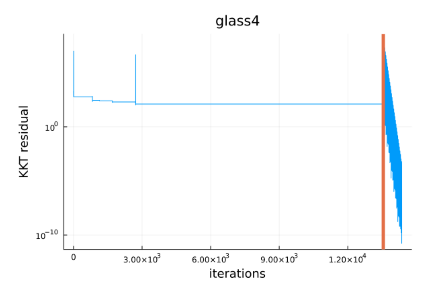
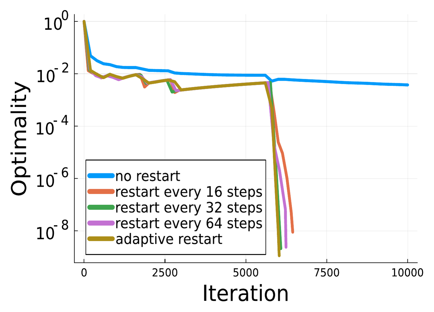
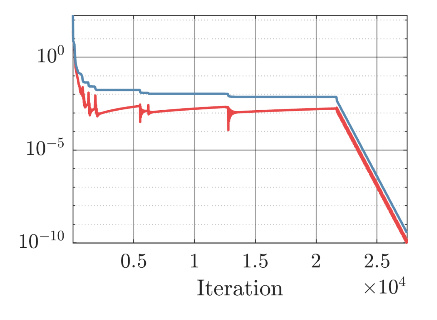
Figure 1. (a) from Lu & Yang (2025), (b) from Chen et al. (2025), (c) from the source cited in §1 of the paper.
Section 2
Intuition of the afterimage: a simple 2D LP
The entire mechanism already shows up in an LP with two variables, one equality constraint, and a single number \(\varepsilon \ge 0\) on the right-hand side.
\[ \min_{x \,\in\, \mathbb{R}^2_+} \; x_1 \quad \text{s.t.} \quad x_1 - x_2 = \varepsilon \]
primal. The solution is \((\varepsilon, 0)\) for every \(\varepsilon \ge 0\).
\[ \max_{y \,\in\, [0,\,1]} \; \varepsilon\, y \]
dual. At \(\varepsilon = 0\) every \(y\) is optimal. At \(\varepsilon > 0\) only \(y = 1\) is.
At \(\varepsilon = 0\) the dual has a whole segment of solutions, and ADMM stops anywhere on it. At \(\varepsilon = 0.1\) only one point of that segment is still a solution, yet the method behaves almost the same, and the optimal set of the left problem becomes an afterimage of the right one.
In each video the static background is the residual field of the problem, colored by the size of the step the method would take from that state, with dark meaning small, and three ADMM runs from the same three starts are drawn on top of it.
Figure 2. ADMM with \(\sigma = 1\). The two fields barely differ, although the solution sets do.
The reason is that the method only ever sees the residual field, the step \(\delta_\theta(z) := T_\theta z - z\) it would take from each state, and this field changes continuously with the data even when the solution set does not. So the method crawls along a segment that is no longer there, and the length of the crawl can be computed:
\[ \text{plateau height} \;=\; \frac{\varepsilon}{\sqrt{2}}, \qquad \text{plateau length} \;\approx\; \frac{2\sigma}{\varepsilon}\ \text{steps} \]
With \(\sigma = 1\) that is 202 steps at \(\varepsilon = 10^{-2}\) and 20,003 at \(\varepsilon = 10^{-4}\), on a problem with a unique solution.
Section 3
Formalizing the afterimage principle
To make this precise, we look at a region \(R_\varepsilon\) of the state space, divide the step the method takes by the distance still to be covered, and keep the worst ratio:
\[ \rho_\varepsilon \;:=\; \sup_{z \in R_\varepsilon} \frac{\lVert \delta_{\theta_\varepsilon}(z) \rVert}{\operatorname{dist}(z, \operatorname{Fix} T_{\theta_\varepsilon})} \;\longrightarrow\; 0 \]
a slow region family
Because the methods are averaged maps, the step never grows along an orbit, so an orbit that starts in the region keeps a fixed fraction of its distance for at least about \((1-\beta)/\rho_\varepsilon\) iterations, up to constants of the method's metric. This is a lower bound on the length of the stall, not an estimate of it.
Center and petals
Bounding the supremum directly is hard, so we build slow regions by comparing two problems. The center is the problem we actually solve, and a petal is a nearby problem that we are free to choose, which may even be infeasible or have no fixed point.
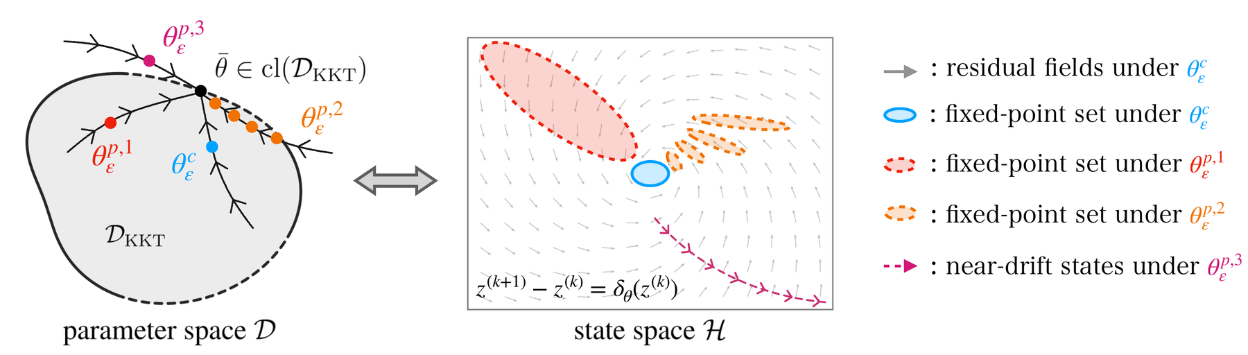
- Take the states where the petal's field equals its drift \(v_{\mathrm p}\), its smallest possible step (\(v_{\mathrm p} = 0\) when the petal has solutions).
- The data are close, so the center's field there differs from \(v_{\mathrm p}\) by at most a multiple of the data gap.
- By construction, the center's own solutions are far from those states, compared with the gap.
- So the center's step there is at most \(\lVert v_{\mathrm p}\rVert\) plus the gap, while its distance to its own solutions is large, which makes \(\rho_\varepsilon\) small. Thickening the set turns it into a region.
Section 4
Three geometric instances of the afterimage principle
Step 3 asks for the center's solutions to be far from the petal states, and the paper proves three ways in which this happens. Each animation sweeps the parameter toward the limit.
Figure 4. Red is the petal and blue is the center.
Section 5
A gallery of more afterimage regions in conic LP
Escape to infinity in an LP, under PDHG
\[ \min_{x \,\in\, \mathbb{R}^2_+} \; x_2 \quad \text{s.t.} \quad -x_1 + \varepsilon\, x_2 = 1 \]
center. \(\varepsilon > 0\), solved only by \(x = (0,\, 1/\varepsilon)\), which escapes as \(\varepsilon \to 0\). petal. \(\varepsilon = 0\), infeasible, so PDHG has no fixed point, only a drift.
Two petals, two plateaus, one SDP run
\[ \min_{X \,\in\, \mathbb{S}^2_+} \; X_{22} + \varepsilon^2 X_{11} \quad \text{s.t.} \quad 2X_{12} - X_{22} = \varepsilon^3 \]
center. \(\varepsilon > 0\) in cost and right-hand side. petal 1. both zero, so the problem is \(\min X_{22}\) s.t. \(2X_{12} = X_{22}\), whose ADMM fixed points form a ray. petal 2. only the right-hand side zero, which leaves a segment.
Section 6
Two real-world problems
Neither problem was built to show the effect. Both start from the solver's default zero state, and the petal is read off the run rather than designed.
Reading the petal off the orbit. On a plateau the primal residual is essentially zero and the dual pair stops moving. The frozen pair makes the plateau state a fixed point of a nearby problem that differs from ours only in its cost, the projection of the nominal cost onto what the frozen slack allows. Nothing is chosen by hand.
BQP-20q, the moment relaxation of a binary quadratic program, the model behind max-cut
With twenty binary variables, the cone is \(\mathbb{S}^{211}_+\) and there are \(m = 16{,}171\) constraints. The relaxation is exact and strictly complementary, so convergence is locally linear. Even so, 71% of the 27,756 iterations lie on four plateaus, with primal rank 7, 4, 3 and 2 before the rank-one tail: face selection four times in a row.
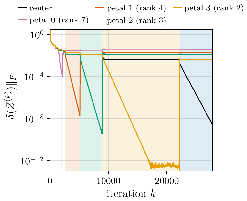
Figure 6. The orbit is solving one petal after another. The black curve is our residual, which is the step norm, frozen on each plateau. The colored curves are the residuals of the four petals: on its own plateau each one collapses, to \(10^{-8}\) and below on plateaus 1 to 3, while the others stay large.
STOCFOR1, a forestry planning LP from Netlib
The instance has \(117\) constraints and \(165\) variables after slacks and is used unscaled. From the zero start, ADMM joins a segment of petal fixed points at iteration 1,727 and rides it until 73,474. The petal cost is 0.14% from the real one in norm, and the change is readable: it cuts the seven timber-revenue coefficients to 37–39% of nominal.
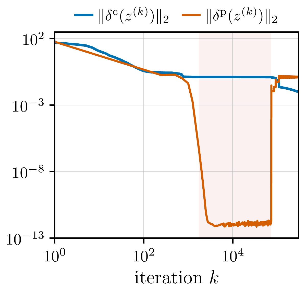
Figure 7. The orbit is solving the petal, not our problem. Across the shaded ride our residual (blue) is frozen at 0.129, while the petal's (orange) decays to \(10^{-11}\). The distance to our solutions falls only from 12,589 to 3,324.
| instance | plateau | modulus bound / measured | prediction / observed |
|---|---|---|---|
| STOCFOR1 LP |
\(k = 1{,}727\)–\(73{,}474\) | \(2.6\!\times\!10^{-5}\) / \((1.0\text{–}2.6)\!\times\!10^{-5}\) on \(k \le 60{,}000\), where the bound applies |
horizon 48,738 / 48,741 exit 73,474 / 73,474 |
| BQP-20q SDP |
four plateaus, 19,800 of 27,756 |
\(2.2, 2.5\!\times\!10^{-4}\) / \(2.2, 2.5\!\times\!10^{-4}\) plateaus 1 and 2 |
three exits, each within 1 iteration, forecast 1,142–7,170 ahead |
What this settles. Afterimage regions occur in problems not built to show them, orbits from the standard start enter them, the petal is computed rather than invented, and its face geometry predicts when the stall ends.